Table of Contents
a place for my sketchy notes on the project…
more info
- my initial research report: pix_research_report
- which evolved into: research_report_pix
this project has two main parts, the creation of a tool, and the explorations made using that tool.
creating the tool
at the moment, effort is focused on creating the tool. this entails a lot of software engineering glue problems, which probably aren't interesting to most.
some of my starting assumptions / decisions:
- using ogre as a renderer (with the goal of creating a reuseable ogre object which can render a given attractor)
- using pyOgre as a glue/scripting layer. this is based on my experience at the xmed-k workshop, to explore the apparent benefits of being able to work at two different levels of abstraction (scripting in python, coding in c++).
- using wxWidgets as a GUI library (actually wxPython, the Python bindings to wxWidgets)
embedding
my first (quite boring) problem was trying to embed an ogre window into a wxPython app.
embedding in this case means having the ogre render into some area within an existing window, alongside some wxWidget controls. the alternative (which i have since fallen back to) is to have the ogre output appear in it's own, separate window.
the root of the problem (that is, why i didn't just DO IT), was that in order for two libraries (wxWidgets, and OGRE) to render into the same window (in an X Windows environment), they need to share some quite low-level information about the window. specifically, because X Windows works with a client/server model, the two libraries need to do all of their communication with the X server over the same communication channel. because i am using python as a glue language, information can only get between wxWidgets and OGRE via their respective python bindings, and python itself. the communication chain looks something like: wxWidgets → wxPython → Python → pyOgre → OGRE. it turns out the the specific information that OGRE needs in order to render into a window that has been created by wxWidgets is lost at the wxWidgets → wxPython transition (quite early).
it's hard to write about decision which you now know are false… anyhow.
in theory, the information isn't exactly lost, but the access layer, wrapped around the wxWindow object, doesn't provide the means to access the needed information. this suggests a few solutions.
i thought i had three different options.
- modify the wxPython bindings, giving access to the needed information.
- modify the pyOgre bindings to unwrap the wxWindow object and access the necessary information
- create a third library which does the unwrapping. returning the needed information in a form which can be passed to pyOgre.
in both cases 1 and 2, the changes necessary would be overly specific. that is, the addition to wxPython would be obviously a hack to achieve something in pyOgre, and vice versa. for this reason i looked into option 3.
it turns out, that in order to get access to the wxWindow object from a third library (or even from pyOgre) i would need to include a considerable chunk of the source of wxPython. this destroyed any benefits of making an independent library. it would be less problematic to create a patch to wxPython to expose the necessary information.
but needing people to recompile wxPython is a requirement i would rather not impose, so for the time being i am settling with having the ogre output appear in a separate window.
interfaces
finally getting on to working with the interface components of wxPython.
the layout of the interface is still pretty sketchy in my mind. but one thing i am pretty sure i want is a way to easily change each of the coefficients. at first i was thinking of sliders, but these take up a lot of space (there will be a lot of them) and it's not really clear if the graphical representation of the coefficients will be useful (in a sense each coefficient represents an orthogonal axis in a high dimension number space, but at best, horizontal and vertical sliders can only really represent two dimensions with any clarity).
so, without sliders, i guess simple number boxes will be the easiest. the latest problem with this is that the default number boxes in xwWidgets (SpinCtrl) only deal with integers. i will be dealing with floating point numbers around +/- 1.
perhaps it is possible to implement a custom control. this was the response to a similar query about floating point sliders, http://lists.wxwidgets.org/archive/wxPython-users/msg11406.html
actually, looking closer at the demo code, the SpinButton demo displays the text manually with a text box. so making a custom controller should be easy. the spin button will still store integers internally, but i think i will take something of a fixed-point approach, and just specify a multiplier that is applied to the internal SpinButton value to generate a fractional value.
exploring the space
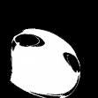
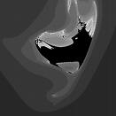
i just got to the state of being able to evaluate the maps. i don't have it connected to OGRE yet, so i don't have any visualisation of the actual attractors, but i was able to skip ahead quite a bit and make these plots of the fractal dimension for different starting positions. it is black where the computation fails.
* highf-100.png:
note from the future (!!): i realise now that this is actually a plot of the basin of attraction (i was changing the initial value for each point in the image, not the constants of the equation). this is also why the fractal dimension isn't changing very obviously. much much later, i do a plot of the fractal dimension when actually changing the constants and the results are more interesting.
to save computation time i did some plots without calculating the fractal dimension. instead just seeing if the computation lasts for 500 steps or so without failing.
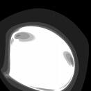
this is a plot of different values of the starting point. [x,y,0] where x and y are in the range [-1.5,1.5]
* highf-xy256.png:
* highf-xz256.png:
* highf-yz256.png:
as an aside i realised that different starting points is just the same as choosing different coefficients, since the effect of choosing a different starting point could also be achieved by shifting the graph by a constant offset, which can be achieved by changing the coefficients. wow, this is super-wrong. although this assumption kind of holds with a normal polynomial, if you start iterating, it all falls down.
17 Dec 2006
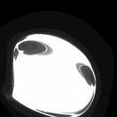
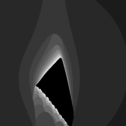
i was thinking a bit about the way the mandelbrot set works. it's quite similar to what i have been rendering here. the central part of the mandelbrot set represents the inputs to a particular iterative function where the values don't spin off to infinity. the rings around this central area are indicating how many steps you need to iterate before the value increases beyond some threshold. i realised that by doing a similar kind of test on the function i have been working with, i could considerably decrease the number of iterations i would need to calculate. here is a 512×512 rendering of the same xy slice as above (rendering time was about 352 seconds):
* highf-xy512esc.png:
you might notice that the white area isn't as detailed as it was above. this is because i set the maximum number of steps to evaluate too low. as you get closer to the fringes, this low threshold smoothes out the areas where the iteration might tend toward infinity quite slowly as it teeters on the border between stability and instability. i think with the mandelbrot set there is some optimisation where the step count is only increased in these tricky areas. this would be useful here because if we (for example) double the step size, then it means all of the white area will take twice as long to compute. i'm not sure how to make such an optimisation in our case.
here is a rendering with the maximum numbers of steps clamped to 20 (earlier it was just 10). rendering time was 612 seconds.
* highf-xy512esc20.png:
as the image is normalised, the higher step count decreases the brightness of the rings. i think i'll start rendering the white area black now to prevent this.
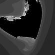
i changed my program to actually plot variations in the coefficients, rather than the initial values. this is a plot of the first coefficient of the x equation (the constant term), against the second coefficient (the x term). the fact that the two terms are of different degrees (0, and 1) is, i think, the reason why it appears to be stretched in one dimension. changes to the x term probably have a much bigger impact on the function than changes to the constant term.

* highf-c00-01-512esc20.png:
here is a plot of the constant term from the x equation against the constant term of the y equation;
* highf-c00-10-512esc20.png:
i just rendered a short animation of the above plot, moving along the constant term of the z equation. since things are happening quite fast in the detailed fringes, here is the middle part of the animation larger and in slow motion . – pix - 19 Dec 2006
the x constant against the z constant:

* highf-c00-20-512esc20.png:
the y constant against the z constant:

* highf-c10-20-512esc20.png:
the x term of the x equation against the x term of the y equation:

* highf-c01-11-512esc20.png:
the same but from the x and z equations:

* highf-c01-21-512esc20.png:
and finally the y and z equations:
* highf-c11-21-512esc20.png:
now that i've seen these images, i'm a bit more content to look into the behaviour of lower degree polynomials, to see if the results are any less 'complex'.
this is a degree 1 attactor (that just scraped in with a fractal dimension of 1.. so it probably just looks like a line). this is the y term of the x equation plotted against the y term of the y equation. obviously much simpler looking. i wonder how this would look as an animation. actually, even though there are far fewer terms involved (8 coefficients versus 168), this still took 280 seconds to render (about half the time of the last few degree 5 renders).
* deg1-c02-12-e20.png:
if you are also interested in how this might look as an animation, look here. it is the same slice as above, animated by moving the z term from the z equation. it took 21730.27 seconds to render (overnight).
by the way, apparently it is possible to show (although i am yet to find a good reference) that the colour bands in the mandelbrot set are all connected. does that make the fact that the colour bands are crossing over here interesting? in a purely aesthetic sense it is interesting that this plot seems to imply space (as if looking into a tunnel) but it is the same kind of plot as all of the other images on this page.
18 Dec 2006
since i haven't mentioned anywhere here what the actual equations are, i'll quickly explain it for this simple degree 1 case. the above is the result of three equations:
- x' = A + Bx + Cy + Dz
- y' = E + Fx + Gy + Hz
- z' = I + Jx + Ky + Lz
the constants A through L are determined by brute force random search, but more on those in a sec. we start with x, y, z = 0. we determine the new values for x, y and z (x', y' and z') by substituting the existing values for x, y and z into the above equations, giving us our new values.
we find the constants A through L by randomly selecting values, and checking if the resulting system fits certain criteria. some criteria can be tested for automatically. one important criteria is that the iteration doesn't produce values that spin off to infinity. imagine the equation x' = 1 + x*2. the first few values you get would be: 0, 1, 3, 7, 15, 31, 63, 127, 255, 511, 1023… and they will just keep getting bigger until eventually they are too big to work with. testing for this is pretty easy, and normally the values stay quite small, so you don't even have to wait for the numbers to get very big. you can catch them as soon as they get bigger than 5 or so.
other criteria are a little more complicated. one useful one is called the fractal dimension, and this is a value which describes roughly some characteristics of the resulting series of values. without going into a lot of detail, you can kind of determine if the resulting points generally tend to clump into one spot, or spread out into a line, fan out into a plane, or balloon into a space, or something in between. annoyingly though it is quite costly to determine the fractal dimension accurately, because you need to compare lots of pairs of points from the attractor. you can however get a bit of an idea by doing a random sample, but this introduces variation into your results. this is why the first plot i did using fractal dimension (above) looks noisy.
so anyhow, i just ran my random constant-finding routine a few times until i found some settings which had a high fractal dimension. 1.0 was the best i could get so far. the plot you see above is the result of testing, for a range of constants close to the set i found, how many iterations it takes for the resulting point (x.y.z) to get a certain distance away from 0,0,0. the black regions are those regions where the points stay near 0,0,0 indefinitely (or for as long as the program bothered testing). the very center of the image represents exactly the list of constants which my hunt returned. areas to the left and right of this point have lesser or greater values for the C constant, respectively. areas above and below the center have lesser or greater values of G respectively. in the animation, it starts by rendering results for a lesser value for L and finishes with a higher value. the choice about which constants to vary is mostly guided by the aesthetic outcomes.
19 Dec 2006
previously i haven't been able to get psyco (an optimising compiler for python) working with my code. i was able to partially remedy this, and the last animation i rendered (32 frames at 512×512) completed in 9541 seconds, or 298 seconds per frame, on average. so psyco has halved rendering time.
29 Dec 2006
i have some first results of rendering the actual 3d attractor which all of these parameter-space plots have been related to. unfortunately, the particular attractor i have been analysing, turns out to not be very interesting to look at (just a wobbly loop), so no pictures yet. the boringness of the attractor is possibly because i only used the fractal dimension to choose the attractor. in the sprott book (and my original applet), the luypanov (sp?) exponent is also used.
my plan now is to get the the point where i can interactively fudge the values of the attractor and get a realtime display of the resulting attractor, with the results of metrics such as the fractal dimension. ideally, it would be possible to do a parameter space plot, and then click somewhere on the plot to see the attractor associated with a given point in parameter space.
it would be also interesting to have an automatic parameter fudger (like my applet) but with more parameters controlling the automatic search. for example, hill climbing to maximise some metric. in the sprott book, there is some data correlating how highly people rated a given attractor and cross referenced to the values of the two metrics. there was an obvious maximum for particular values of both. it would be interesting to hunt towards attractors that had these 'optimal' properties.)
20 Jun 2007
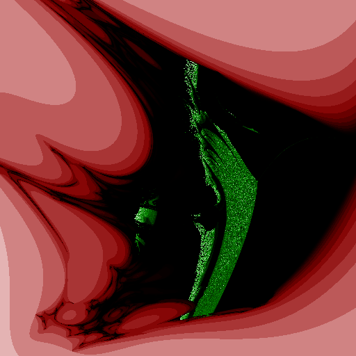
lots of changes in the last few months, but i just wanted to upload this neat new render. i made a normal escape plot for a slice of an attractor (in red, lighter colours mean quicker escape), and then overlayed a plot of the fractal (correlation) dimension (green, lighter colours mean higher dimension).
so, to describe a bit more. the black and green areas are where the map doesn't just spin off to infinity, but keeps returning values. in the black areas, the fractal dimension is very low, so it is possible that the map just returns a small number of points over and over again. in the green areas, the fractal dimension is higher (and highest where the green is lightest). the points with highest dimension probably produce points in a voluminous cloud, or at best a sheet. the darker green areas possibly producing points arranged as lines.
it would be really interesting to be able to click around on this image and see the attractor that each point represents. i'm not sure yet if that will make it into the research or if it will just be listed as a future direction.
Yet another animation
Oh, and there is this neat new animation. First some ramblings. I was showing the parameter plots above to Tim Boykett, and he pointed out an important assumption that I was making. The plots are specifically plotting the presence of attractors that just happen to have 0,0,0 in their basin of attraction (because the function doing the escape-plot always uses 0,0,0 as the starting point). To investigate how important this assumption was, I made an animation of parameter plots for changing initial values. The base attractor is the one used in all of the images called “highf” above. At the start of the animation, the initial value used for the parameter plots is -1,0,0, and by the end it is 1,0,0. In the middle of the animation, you should see a frame that looks like highf-c00-01-512esc20.png above (only with the black part filled in white, and rotated 90 degrees counter-clockwise - the renderer has changed a bit) when the initial value hits 0,0,0.
(this is here twice because the second one, which is the right way to link images with thumbnails, results in a slightly corrupted animation)
twiki era cruft
   png highf-c00-20-512esc20.png manage 22.2�K 17 Dec 2006 - 21:14 pix
 � png highf-c00-10-512esc20.png manage 18.5�K 17 Dec 2006 - 21:12 pix
 � png highf-c11-21-512esc20.png manage 11.7�K 17 Dec 2006 - 21:25 pix
 � png highf-100.png manage 4.8�K 15 Dec 2006 - 17:32 pix
 � png deg1-c02-12-e20.png manage 11.8�K 17 Dec 2006 - 23:05 pix
 � png highf-xz256.png manage 3.9�K 15 Dec 2006 - 17:29 pix
 � png highf-c00-01-512esc20.png manage 18.5�K 17 Dec 2006 - 21:10 pix
 � png highf-yz256.png manage 3.7�K 15 Dec 2006 - 17:49 pix
 � png highf-xy512esc20.png manage 16.2�K 17 Dec 2006 - 15:00 pix
 � png highf-c01-21-512esc20.png manage 18.9�K 17 Dec 2006 - 21:23 pix
 � png highf-xy512esc.png manage 12.5�K 17 Dec 2006 - 14:12 pix
 � gif highf-zanim.gif manage 308.5�K 19 Dec 2006 - 06:53 pix
 � gif deg1anim.gif manage 520.9�K 18 Dec 2006 - 08:32 pix
 � gif highf-zanim-slow.gif manage 382.7�K 19 Dec 2006 - 13:25 pix
 � png highf-xy256.png manage 3.6�K 15 Dec 2006 - 17:28 pix
 � png highf-c01-11-512esc20.png manage 20.9�K 17 Dec 2006 - 21:22 pix
 � png highf-c10-20-512esc20.png manage 15.4�K 17 Dec 2006 - 21:32 pix

�
Libarynth > Libarynth Web > TWikiUsers > PiX > PixStrangeAttractor r15 - 16 Feb 2007 - 18:11 -


